
A rocket nozzle jet: from exit conditions to plume structure
A parametric bell nozzle links a supersonic plume to exit-plane measurements, with numerical sensitivity and model limits kept explicit.
01
What should be checked beyond the nozzle exit?
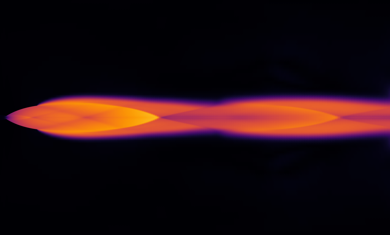
A nozzle exit value alone does not describe the downstream plume. This study connects the exit plane to the expanding high-Mach region and its downstream narrowing. The engineering purpose is to identify where pressure and velocity should be inspected before choosing a higher-fidelity analysis. It is a single-condition baseline, with no redesign or efficiency improvement claimed.
02
A defined model and operating condition
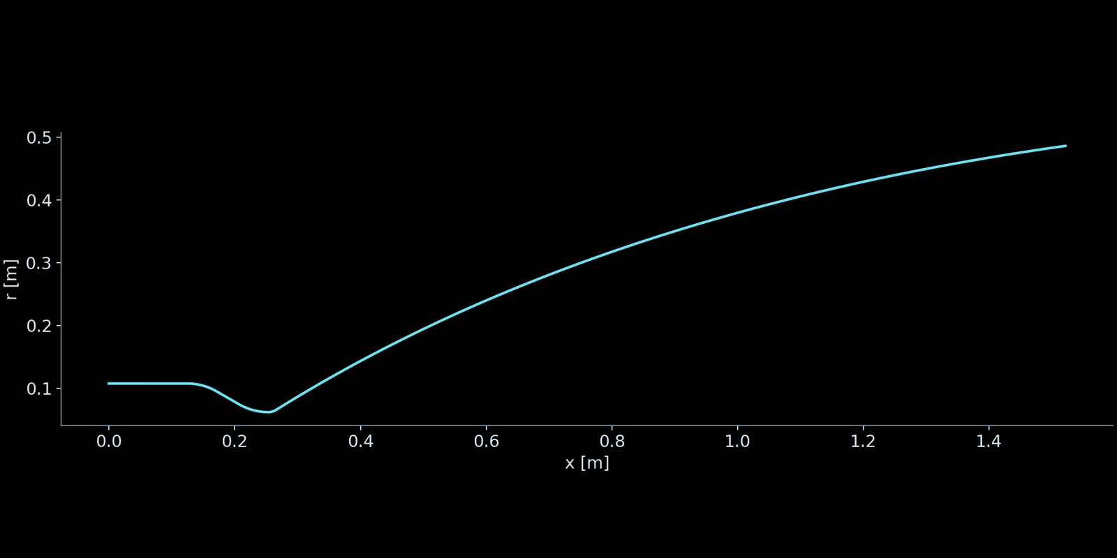
The parametric bell contour has a 124.46 mm throat diameter and an exit-to-throat area ratio of 61. The axisymmetric Euler model uses a single gas with constant specific heats: heat-capacity ratio 1.22 and gas constant 355 J/(kg·K). Inlet total pressure is 3.20606214 MPa and total temperature is 3000 K; ambient static pressure is 2.000 kPa. The 20,840-cell continuation covers 32–50 ms with a 20 microsecond physical step and second-order spatial reconstruction. The drawing mirrors the computed meridional half-plane for viewing; it is not an independently computed lower half or a three-dimensional result.
| Parameter | Value |
|---|---|
| Throat diameter | 124.46 mm |
| Exit / throat area ratio | 61 |
| Inlet total pressure | 3.20606214 MPa |
| Inlet total temperature | 3000 K |
| Ambient static pressure | 2.000 kPa |
| Heat-capacity ratio / gas constant | 1.22 / 355 J/(kg·K) |
| Physical time step | 20 μs |
| Continuation interval | 32–50 ms |
03
The mesh behind the result
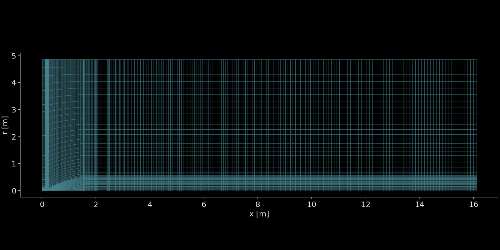
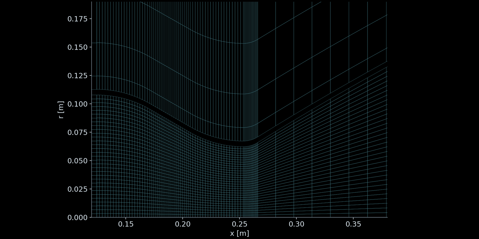
The actual 20,840-cell meridional mesh covers the nozzle interior, the region outside its wall and the downstream plume. The external domain extends 15 exit diameters downstream and 5 exit diameters radially. The throat view shows how the mesh follows the curved wall and concentrates axial stations around the throat. This is the mesh used by the continuation, not a schematic. Cell clustering resolves geometry and gradients; it does not establish mesh independence or represent a viscous boundary-layer model.
04
Read the plume and pressure together
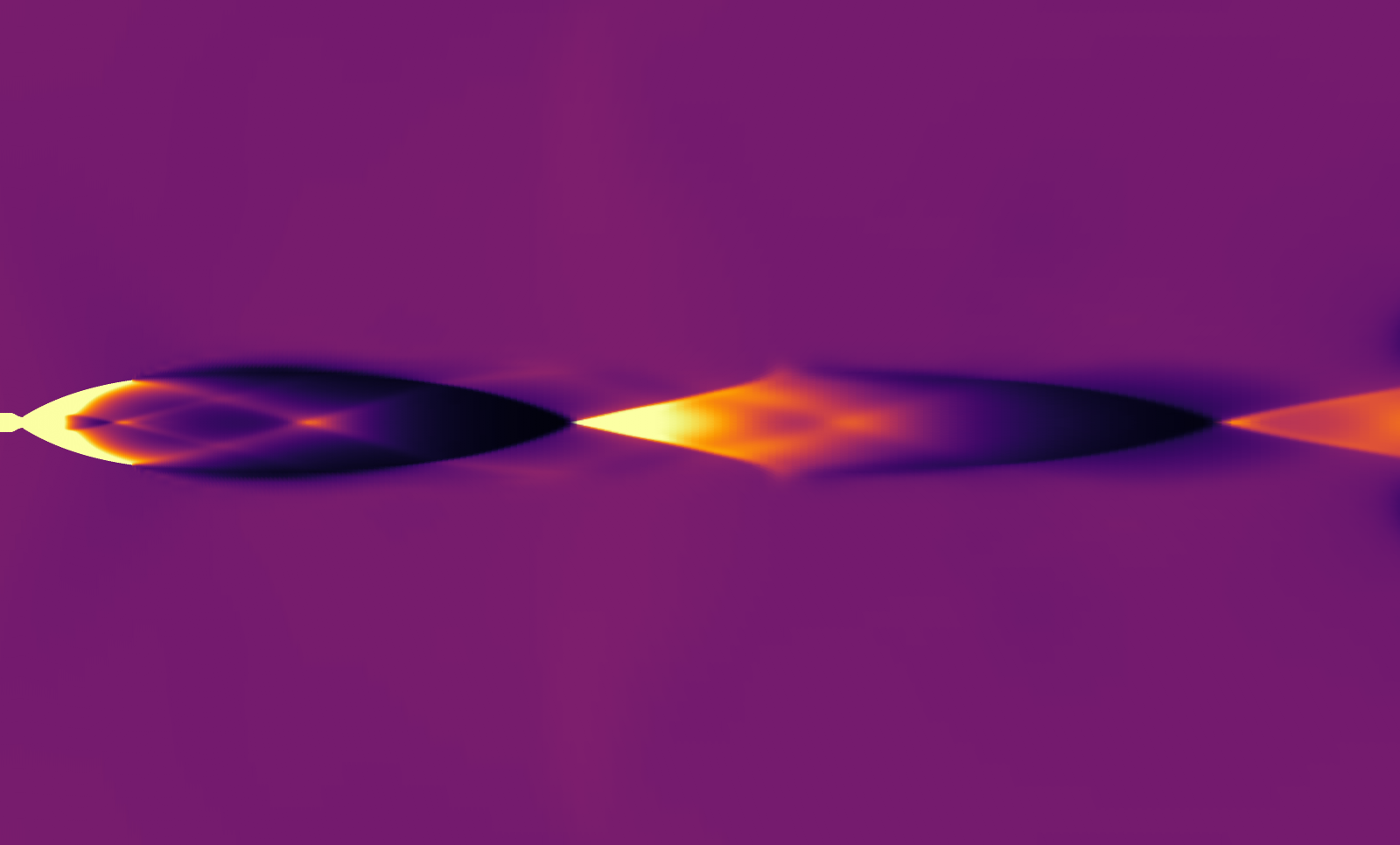
At 50 ms the high-Mach region spreads outward beyond the exit near x = 1.52 m, then narrows farther downstream. The companion pressure-ratio map provides a second view of this spatial structure. Its scale is static pressure divided by the 2.000 kPa ambient pressure; values above 3 are saturated. Mach is dimensionless and uses a fixed 0–8 color mapping. These are stationary snapshots of an unsteady calculation. Moving across the image means moving through space, not watching time advance. The visible structure identifies regions for closer inspection; it does not quantify mixing, thermal loads or thrust. The full-domain figures use a dark sequential color map, without axes or colorbars; brighter tones indicate larger values. Use the numerical table and centerline curve for quantitative reading.
05
Exit measurements at 50 ms
Integration of the final saved field gives 24.1283 kg/s exit mass flow, area-mean Mach 4.6994, area-mean static pressure 3.63447 kPa and area-mean speed 2890.08 m/s. Mass flow integrates density times axial velocity over the axisymmetric exit area. The other values are area means, not centerline peaks or mass-weighted means. The mean exit pressure exceeds the configured ambient pressure; the expanding region just outside the exit is consistent with that pressure mismatch. A numerical baseline can therefore guide where to inspect the plume without implying a tested engine performance.
| Metric | Value |
|---|---|
| Mass flow [kg/s] | 24.1283 |
| Area-mean Mach [1] | 4.6994 |
| Area-mean static pressure [kPa] | 3.63447 |
| Area-mean speed [m/s] | 2890.08 |
06
Locate pressure changes along the plume
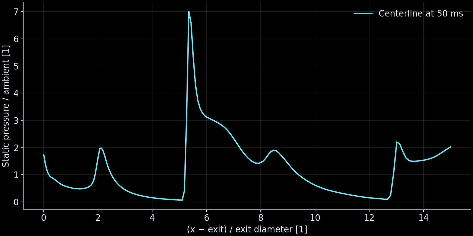
At 50 ms, the centerline pressure curve resolves spatial changes hidden by an exit-area average. Distance is measured from the exit and divided by the exit diameter; pressure is divided by the 2.000 kPa ambient value. Low-pressure intervals and subsequent pressure rises identify expansion and compression regions to inspect alongside the contour. Unlike the contour capped at a pressure ratio of 3, this curve retains the exported values. It is a spatial profile at one time, not a pressure history or a measure of oscillation frequency.
07
Separate temporal variation from grid sensitivity
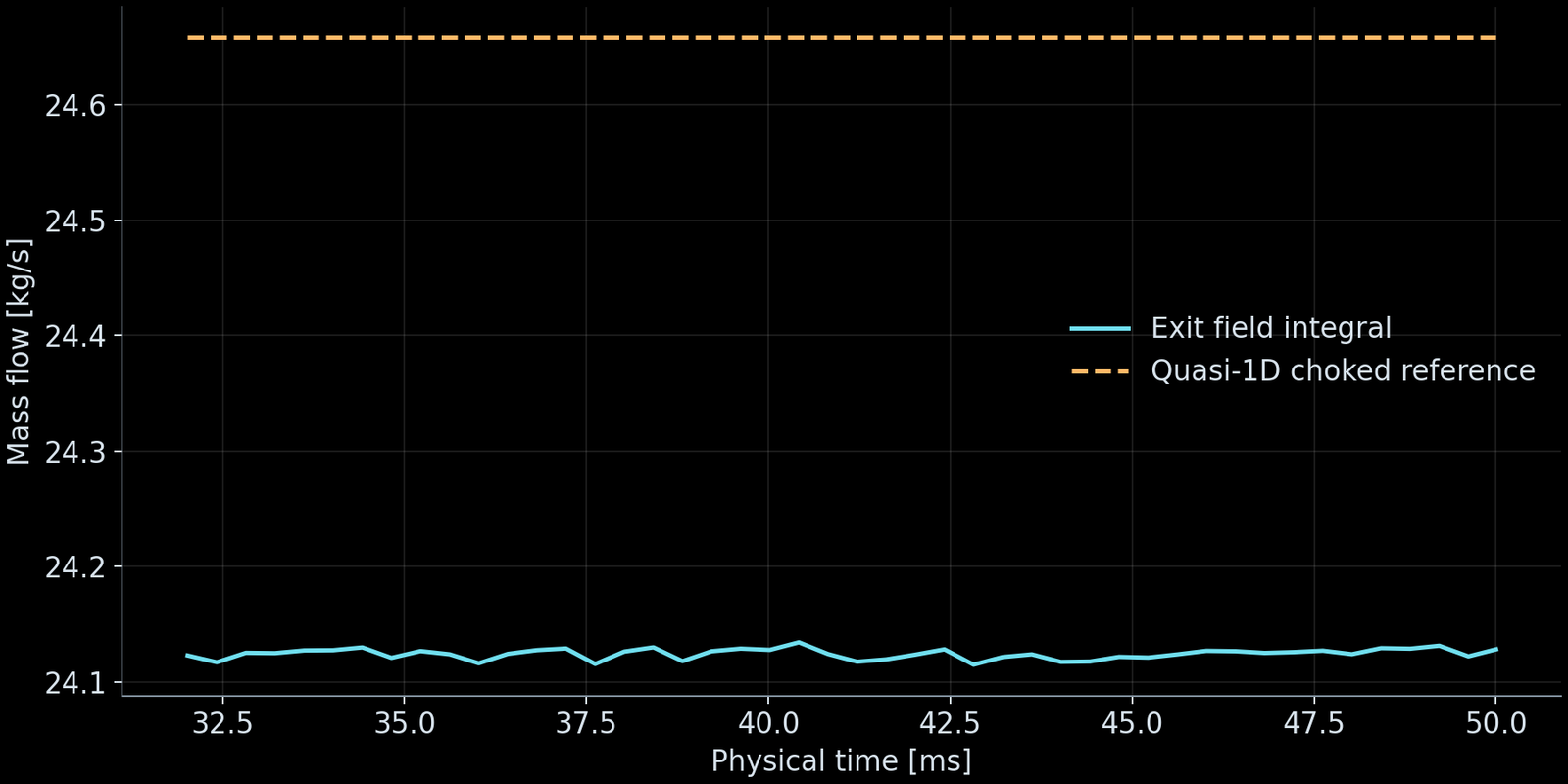
The history shows 46 exported samples between 32.02 and 50 ms. Its small variations must be read against the axis ranges; stability of these exit averages does not establish stability everywhere in the plume. An earlier same-time comparison at 16 ms used 10,312 and 20,840 cells: exit mass flow was 23.9924 and 24.1264 kg/s. On the finer grid it was 24.1225 kg/s at 32 ms. Grid change and time extension answer different questions and should not be combined into an improvement percentage. The two-grid comparison is not a grid-independence certification. The dashed line is the quasi-one-dimensional choked-flow reference, 24.6576 kg/s, not a measurement. The final computed flow is about 2.15% below it. The 46 sampled values span 24.1150–24.1344 kg/s; these small fluctuations are distinct from the offset to the reference.
08
Use the baseline to choose the next validation
The final exit integrals were recalculated from the saved conservative fields and checked against the exported metrics. The run log records normal completion, and its diagnostic summary reports the configured numerical checks passed. This verifies the provenance and internal consistency of these reported outputs; it does not establish experimental accuracy. The inviscid model contains no combustion, turbulence, heat transfer or species mixing. The parametric contour is not a manufacturing geometry. Use this baseline to choose plume sampling locations and to frame a viscous, reacting or thermal study when those quantities drive the design. The selected later continuations inherit an earlier startup that did not pass its configured checks; passing continuation checks does not validate that entire trajectory.
FILM
Beyond the nozzle
The original Dashboard video is played without changes to its frames, colorbar or playback speed. It covers 0–50 ms in 129 frames at 10 fps, lasting 12.9 seconds. The first frame is the configured initial field; later frames are computed states with unequal physical sampling intervals. The first-order 0–12 ms startup did not pass its numerical checks; subsequent continuations do not validate the full trajectory.
Syntrivora
Start with a defined physics question
Discuss operating conditions, required metrics and validation scope.