ONERA CRM-HL high-lift CFD

HLPW-5 Case 2.4 · Loads, separation, and near-stall flow

A CFD study of the ONERA-LRM-LDG-HV landing configuration, linking lift development to surface pressure, multi-element wakes, and three-dimensional separation.

Public benchmarkIndependent simulationHLPW-5 · Case 2.4

High-lift aerodynamicsONERA-LRM-LDG-HVRANSNear-stall flow

00 / Context

Can a practical CFD workflow remain credible as a high-lift wing approaches stall?

The deployed slat–flap system creates strong pressure gradients and interacting wakes. The nacelle, pylon, chine, and tail add three-dimensional flow interactions. This study follows how these structures redistribute loading and drive separation as incidence increases.

What evidence is needed before a high-lift CFD result can support an engineering decision?

2.4

HLPW-5 test case

prescribed incidence angles

planned mesh levels

pressure / profile stations

Study status

The calculation matrix and post-processing specification are defined. Aerodynamic results will be added after convergence, mesh-sensitivity, and statistical checks.

01 / Define the decision before running the solver

A useful benchmark tests both performance and credibility

The prescribed Mach and Reynolds numbers establish the flow regime, while the incidence sweep exposes the change from predominantly attached flow to large separated regions. A decision-ready assessment must distinguish physical trends from convergence, mesh, turbulence-model, and solution-path effects.

Ma=0.20,\qquad Re_{MAC}=5.9\times10^6,\qquad C_p=\frac{p-p_\infty}{q_\infty}

Design question	Decision metric
Are the integrated loads stable?	Converged or statistically stationary $C_L$ , $C_D$ , and $C_m$ histories
Is the loading mechanism credible?	Element-level and spanwise $C_p$ distributions
Where does performance deteriorate?	Wall shear, surface streamlines, sectional velocity, and vorticity
Does the conclusion survive refinement?	Consistent trends across at least three related meshes
Is near-stall behavior model-dependent?	Model and steady/unsteady sensitivity at selected conditions

A useful benchmark tests both performance and credibility

A close value of $C_L$ alone is insufficient: pressure errors on the slat, main wing, and flap can cancel. Integrated and local evidence must support the same explanation.

02 / Use a public three-dimensional reference

HLPW-5 Case 2.4 isolates a demanding three-dimensional problem

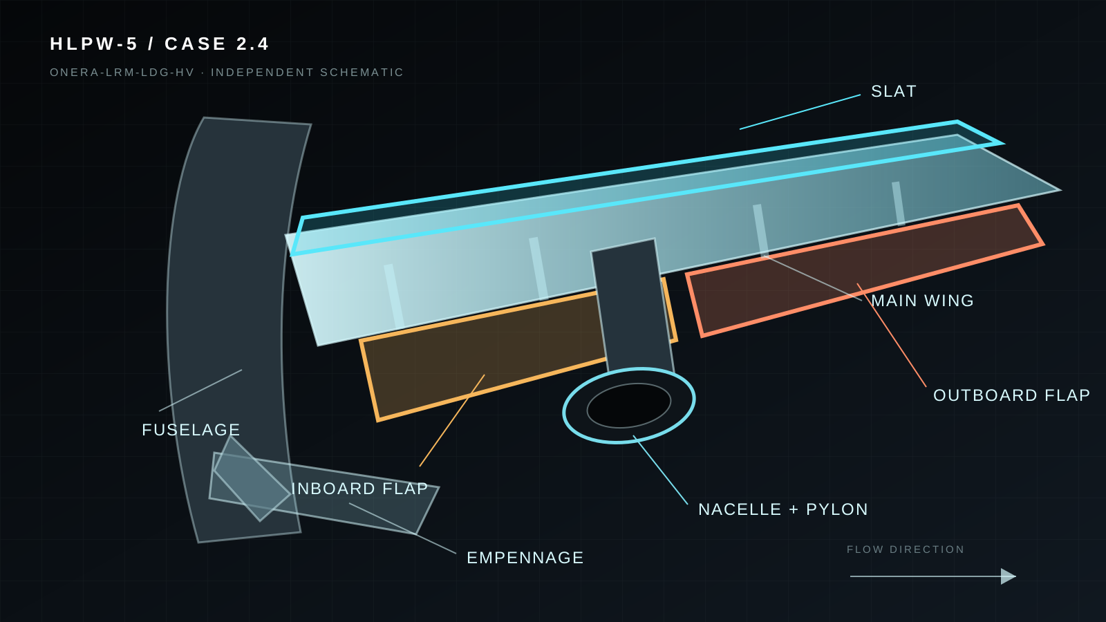
ONERA-LRM-LDG-HV is the full landing configuration in the HLPW-5 Case 2 geometry build-up. It combines the wing-body, deployed slats and flaps, installation details, a flow-through nacelle and pylon with chine, and horizontal and vertical tails. The workshop geometry is evaluated in free air without reproducing the tunnel walls or support system.

Item	Benchmark definition
Official name	ONERA-LRM-LDG-HV
Workshop designation	HLPW-5, Test Case 2.4
Physical article	ONERA 1/19.5-scale full-span LRM-HL wind-tunnel model
Computational geometry	Free-air geometry supplied at full scale in inches
Mach number	$Ma=0.20$
Reynolds number	$Re_{MAC}=5.9\times10^6$
Configuration	Wing-body-slat-flap-nacelle/pylon with horizontal and vertical tails
Primary flow states	$\alpha=7.6^\circ$ attached-flow reference; $19.7^\circ$ near- $C_{L,max}$ reference
Sampling	16 pressure / velocity-profile stations and Case 2 pressure belts

ONERA-LRM-LDG-HV landing-configuration schematic: wing-body, deployed slats and flaps, nacelle–pylon installation, and empennage.

03 / Change one class of influence at a time

A controlled study keeps the comparison interpretable

The first phase keeps the official Case 2.4 geometry fixed and changes one numerical or physical factor at a time. This prevents geometry, model, and mesh changes from being folded into one unexplained load increment.

Factor	Treatment	Purpose
Angle of attack	Seven prescribed Case 2.4 conditions	Track loading and separation development
Mesh resolution	Coarse, medium, and fine at $7.6^\circ$ and $19.7^\circ$	Measure attached and near-stall numerical sensitivity
Flow modeling	Baseline RANS with selected unsteady follow-up	Determine whether a steady closure is adequate
Geometry	Official Case 2.4 baseline held fixed	Keep the study traceable to the public benchmark

04 / Preserve the details that affect the decision

Build a CFD model with consistent scale, geometry, and resolution

Reference consistency

The geometry is supplied at full scale. Length, area, moment center, pressure coordinates, viscosity, and Reynolds-number definition must be converted as one system; mixing model-scale and full-scale references produces plausible-looking but incorrect coefficients.

Geometry fidelity

Slat gaps, flap passages, brackets, fairings, nacelle-pylon junctions, and the chine influence downstream boundary layers and vortices. Every repair, closure, or suppression is recorded.

Targeted refinement

Resolution follows near-wall layers, slat and flap wakes, wing-body junction, nacelle/pylon, chine-vortex path, flap side edges, tail loading, and separated shear layers.

Boundary and numerics

Far-field extent, symmetry, spatial order, initialization path, and force groups are frozen before the mesh study so comparisons remain interpretable.

Freestream conditions and aerodynamic references

The baseline uses full-scale metres and the positive-Y half-model in free air. Prescribed values follow HLPW-5 Test Cases v1.9 (18 March 2024). Derived quantities use an ideal gas with R=287.05 J/(kg·K) and γ=1.4. These settings define the calculation plan; execution records will accompany published results.

Parameter	Value / definition	Basis
Mach / Reynolds number	Ma = 0.20; Re_MAC = 5.9 × 10⁶	Official Case 2.4
Static temperature T∞	518.67 °R = 288.15 K = 15 °C	Prescribed
Absolute static pressure p∞	14.696 psi ≈ 101325.35 Pa	Prescribed; absolute pressure
Sideslip β	0°	Symmetric baseline
Incidence α	7.6°, 10°, 14°, 16°, 17.7°, 19.7°, 23.6°	Official Case 2.4
Reference chord MAC	275.8 in = 7.00532 m	Official reference
Half-model reference area S	297360 in² = 191.8447776 m²	For half-model force integration
Full-model reference area	594720 in² = 383.6895552 m²	For full-model force integration
Moment reference centre	(1325.9, 0, 177.95) in = (33.67786, 0, 4.51993) m	Original CAD body frame
Density ρ∞ / sound speed a∞	≈ 1.225017 kg/m³ / 340.2923 m/s	Derived from p∞, T∞, R, γ
Freestream speed U∞	≈ 68.05846 m/s	U∞ = Ma · a∞
Dynamic pressure q∞	≈ 2837.110 Pa	q∞ = ρ∞U∞²/2
Kinematic viscosity ν∞	≈ 8.080869 × 10⁻⁵ m²/s	ν∞ = U∞ · MAC / Re_MAC
Dynamic viscosity μ∞	≈ 9.899198 × 10⁻⁵ Pa·s	μ∞ = ρ∞ν∞; matched to full-scale Re
Total temperature / pressure	T₀ ≈ 290.4552 K; p₀ ≈ 104190.95 Pa	Isentropic conversion for total-condition inputs

U_\infty=Ma\sqrt{\gamma R T_\infty},\quad \rho_\infty=\frac{p_\infty}{RT_\infty},\quad \mu_\infty=\frac{\rho_\infty U_\infty MAC}{Re_{MAC}}

Boundary types and baseline model settings

Boundary / model	Selected baseline
Far-field domain	Hemisphere with radius 100 MAC = 700.532 m, centred on the MRC for this study. The radius follows workshop guidance; the centre and implementation are study choices. Check load sensitivity to a larger domain.
Outer boundary	Compressible characteristic far field defined by static p∞, T∞, Ma, and α. For inlet/outlet formulations, map the same freestream state according to flow direction at each boundary.
Symmetry, y=0	Zero normal velocity and symmetry conditions for the remaining variables. Remove this boundary for a full model and use the full-model reference area.
Aircraft walls	Stationary, no-slip, adiabatic walls for baseline RANS, including slat, wing, flap, fuselage, tails, and the internal solid surfaces of the nacelle.
Flow-through nacelle	Keep the fluid passage open and coupled to the external flow, with no engine thrust, imposed engine mass flow, or artificial end caps.
Turbulence baseline	Fully turbulent SA-neg with freestream working variable ν̃∞/ν∞ = 3, selected for this study. ν̃ is the SA working variable, not the eddy-viscosity ratio μt/μ. Record the model variant and solver version.
Gas and viscosity	Ideal gas: γ=1.4, R=287.05 J/(kg·K), Pr=0.72, Prt=0.9. Use a rescaled Sutherland temperature law anchored at the tabulated μ∞, with S=110.4 K.
Free-air setup	Exclude tunnel walls and supports. Hold the zero-incidence geometry fixed and rotate the freestream vector to impose angle of attack.

In the original CAD frame, x points aft, y along the positive semispan, and z upward. At β=0 the velocity vector is (U∞ cosα, 0, U∞ sinα). Transform velocity, probes, and moment centre together if import changes the axes. Lift points upward in wind axes, drag downstream, and positive pitching moment is nose-up.

Consistent scale, pressure, and viscosity

Full-scale geometry requires adjusted viscosity to match both prescribed Ma and Re. Standard air viscosity at 288.15 K would give Re ≈ 32.6 million. For gauge-pressure solvers, use operating pressure 101325.35 Pa and far-field gauge pressure 0 Pa; the equation of state uses absolute pressure. Normalize half-model forces by half-model area without doubling the forces.

Sources: HLPW-5 archive, HLPW5_Test_Cases_v1.9.pdf (pp. 1, 3–5), FAQs.html (Q10, Q12, Q17), and geometries.html.

mesh / slots / wake

Evaluation item · slat supports, flap passages, near-wall layers, and wake refinement

Comparison discipline

All configurations use consistent load definitions, physical conditions, extraction procedures, solver version, turbulence-model variant, numerical schemes, and convergence criteria.

05 / Expand one reference condition into a complete matrix

Eleven baseline runs cover the prescribed polar and two mesh anchors

The medium mesh covers all seven official angles. Coarse and fine meshes are added at $7.6^\circ$ for the attached-flow baseline and at $19.7^\circ$ for the near-maximum-lift condition. Model-sensitivity or unsteady follow-up is added only when the baseline evidence identifies a specific need.

Study block	Cases	Primary output
Case 2.4, all prescribed angles, medium mesh	7	Discrete load polar and flow-regime map
Case 2.4, $\alpha=7.6^\circ$ , coarse and fine additions	2	Attached-flow mesh sensitivity
Case 2.4, $\alpha=19.7^\circ$ , coarse and fine additions	2	Near-stall mesh sensitivity
Selected model or unsteady follow-up	As needed	Diagnose unsupported high-incidence behavior

Nominal free-air incidence set

\alpha\in\{7.6^\circ,\;10^\circ,\;14^\circ,\;16^\circ,\;17.7^\circ,\;19.7^\circ,\;23.6^\circ\}

Eleven baseline runs cover the prescribed polar and two mesh anchors

The eleven-run baseline is a reporting plan, not a claim that eleven verified solutions are already complete. Failed starts, convergence extensions, and diagnostic reruns are logged separately.

06 / Connect performance change to its physical cause

Post-processing connects aerodynamic loads to separation mechanisms

Integrated loads

Plot $C_L$ , $C_D$ , and $C_m$ with convergence or averaging windows. Report references, signs, force groups, initialization path, and whether each value is steady or statistically averaged.

$C_L$ / $C_D$ / $C_m$

Planned Syntrivora output · load polar and convergence histories

Local pressure

Extract $C_p$ on the slat, main wing, and flap along the Case 2 pressure belts. Suction peaks, recovery, flap loading, and pressure plateaus test whether integrated loads come from a credible distribution.

$C_p$ / $x/c$

Planned Syntrivora output · element-resolved sectional pressure

Flow topology

Use skin-friction lines, wall-shear magnitude, sectional velocity, and vorticity to connect load changes with attachment, crossflow, wakes, chine-vortex transport, and separated regions.

surface flow

Planned Syntrivora output · surface and sectional flow diagnostics

Post-processing deliverables

Based on the HLPW-5 post-processing instructions and v10 submission templates. These are the planned outputs for this study. Unsteady statistics apply to time-accurate simulations; spectra and vortex visualizations extend the mechanism analysis.

Result	Extraction and presentation
Load polar and components	Report $C_L$ , $C_D$ , and $C_m$ at all seven angles, pressure/viscous lift and drag, and coefficients excluding both tails. Add lift-to-drag ratio and component loads.
Convergence and mesh sensitivity	Retain coefficient and residual histories, including at least the last 25% of iterations for a converged steady run. Compare loads, pressure, separation, and $y^+$ on three meshes.
Pressure and skin friction	Export $x,y,z,C_p,C_f,C_{fx},C_{fy},C_{fz}$ on the Case 2 pressure belts for slat, wing, flap, fuselage, and horizontal tail.
Surface flow and separation	Show total skin friction $C_f=\|\tau_w\|/q_\infty$ and wall-shear streamlines around the root, nacelle wake, flap edges, and outer wing. Use shear direction to identify reverse flow; provide mean fields for unsteady runs.
16 velocity and eddy-viscosity profiles	At each fixed probe $x,y$ , extract $u/U_\infty,v/U_\infty,w/U_\infty$ and $\mu_t/\mu_\infty$ along body-axis $z$ , covering the boundary layer and upstream-element wakes.
Unsteady pressure and load statistics	Record 16 $C_p(t)$ signals and load histories with means, RMS, averaging windows, and sampling intervals. Add PSD, dominant frequency, and $St=f\,MAC/U_\infty$ where useful; check record-length and time-step sensitivity.
Off-body vorticity and vortex structure	Produce vorticity contours on five fixed $x$ planes, with and without mesh overlays. Use curl of mean velocity for unsteady comparisons. Add velocity deficit, total-pressure loss, and Q isosurfaces at consistent thresholds.

Surface pressure belts: use the Case 2 cutters

Use wing rows A–J, seven flap rows, fuselage rows F.A/F.B, and horizontal-tail rows HT.A/HT.B/HT.C. Deployed slat, wing, and flap belts are not coplanar. Case 2 wing row C has no leading-edge dog leg; skip the UNUSED slat row C. Apply the official Case 2 wing, slat, flap, fuselage, and horiztail cutters rather than treating constant-span slices as experimental pressure belts.

16 pressure probes and profile locations

Coordinates come from the Case 2.4 unsteady-pressure template: original CAD body frame, positive-Y half-model, full-scale inches. The listed z is an approximate upper-surface locator. Place pressure probes at the actual deployed-surface intersection at the specified x,y; sample velocity and eddy viscosity along the corresponding z line. Locations stay fixed to the geometry as incidence changes.

Probe	x / in	y / in	z ≈ / in
A.1	1034.9500	137.9135	191.7500
A.2	1071.2212	160.9808	195.4808
A.3	1365.5096	227.1058	183.1173
A.4	1385.4231	128.3423	156.9615
A.5	1421.5757	129.1298	148.0621
A.6	1444.4584	225.9062	167.1960
B.1	1163.5769	379.9615	190.8654
B.2	1203.7442	374.8077	208.4231
B.3	1398.1731	360.8769	205.5577
B.4	1493.6878	361.0165	173.5348
C.1	1699.5212	964.3962	258.4827
C.2	1730.9519	956.0558	258.5019
C.3	1762.3500	949.1462	255.5058
D.1	1799.3942	1152.4692	268.0192
D.2	1821.0673	1152.2827	270.1462
D.3	1842.7404	1152.2058	271.0212

Full-scale metres = inches × 0.0254; 1/19.5 model metres = inches × 0.0254 ÷ 19.5. Apply the geometry’s translations, rotations, or reflections to the coordinates too. Approximate z values require a surface-location check after CSV import.

Download 16 probe coordinates (CSV, inches / metres)

Five off-body vorticity planes

Official CFD views 11–15 use body-axis x = 1095, 1185, 1275, 1485, 1735 in, or exactly 27.813, 30.099, 32.385, 37.719, 44.069 m at full scale. Plane normals follow the body x axis. Keep views and colour scales consistent and save each plane with and without a mesh overlay.

Unsteady sampling record

Record $t^*=tU_\infty/MAC$ , $\Delta t^*$ , transient removal, and averaging duration; $MAC=275.8$ in. Steady-RANS iteration oscillations diagnose convergence and do not define physical pressure spectra. Sample time-accurate signals uniformly at a rate selected for the highest frequency of interest and check aliasing.

References and coordinate provenance

Archive paths: Workshop5/DataForm.html; nominalgrid_unsteadypressures, velocity, eddyviscosity, cpcf, and FM forms under XXX_Lastname_Code_Model_v10/XXX_Case2.4_Lastname_Code_Model/. Probe coordinates are prescribed extraction locations from the Case 2.4 template.

Post-processing connects aerodynamic loads to separation mechanisms

Agreement in an integrated coefficient across runs does not prove correct local loading. Pressure errors on different elements or span stations can cancel, so local evidence is required before accepting the mechanism.

07 / Treat each incidence range as a different prediction problem

Three flow regimes organize the engineering interpretation

The same setup is not automatically equally credible across the polar. Low incidence tests geometry, references, and basic loading; the lift-build-up range tests multi-element interaction; near and beyond peak lift tests separation, unsteadiness, and solution-path sensitivity.

Regime	Angles	Primary question	Publication gate
Attached-flow reference	$7.6^\circ$ and $10^\circ$	Are loads and element pressure stable?	Convergence plus three-level mesh review
Lift build-up	$14^\circ$ , $16^\circ$ , $17.7^\circ$	How do loading and localized separation evolve?	Consistent load and topology trends
Near/post-stall	$19.7^\circ$ and $23.6^\circ$	Is the flow unsteady or model/path dependent?	Averaging and sensitivity evidence

$C_L$ / separation / sensitivity

Planned Syntrivora output · regime map linking loads, separation extent, and numerical sensitivity

Three flow regimes organize the engineering interpretation

A converged residual is not enough near stall. Persistent force oscillation or moving separation requires time-history inspection and, where justified, unsteady treatment.

08 / Verify the conclusion before recommending a configuration

Four checks define whether the comparison is decision-ready

Iteration and statistics

Review residuals, force and moment histories, mass balance, and separation extent. For unsteady runs, record transient removal, time step, averaging interval, and sampling rate.

Mesh sensitivity

Compare loads, sectional pressure, and flow topology on coarse, medium, and fine meshes, together with near-wall resolution and wake refinement.

Reference consistency

Check geometry scale, reference area, mean aerodynamic chord, moment center, coordinate transformations, and coefficient signs.

Experimental comparison

Match configuration, incidence correction, Reynolds number, pressure-belt locations, and averaging definitions before comparing numerical and experimental data.

HLPW-5 official archive HLPW workshop review

Four checks define whether the comparison is decision-ready

Oscillation in a steady high-incidence solution is not automatically a physical time-resolved load. Its numerical and physical origin must be diagnosed first.

09 / Quantify results and their range of validity

Calculation and reporting progress

The benchmark conditions, baseline run matrix, and extraction locations are defined. Load curves, pressure distributions, and flow visualizations will be published with their numerical verification.

Evaluation	Verified result	Design implication
Benchmark identity and conditions	Established from official HLPW-5 material	Defines the reproducible starting point
Geometry preparation record	Planned Syntrivora deliverable	Makes simplifications auditable
Loads, pressure, and flow graphics	Not yet published	No unsupported aerodynamic claims
Three-level mesh sensitivity	Not yet published	Required before interpreting small differences
Experimental validation claim	Not made on this page	Requires a completed comparison and confirmed data-use basis

Calculation and reporting progress

Seven discrete angles do not by themselves locate $C_{L,\max}$ or the stall angle. Additional incidence points and sensitivity to model, solution path, and averaging are required near the peak.

10 / Reuse the verified baseline for focused design work

How the study supports the next design phase

01Demonstrate geometry preparation for a complex multi-element aircraft.
02Show how an attached-flow baseline expands into near-stall analysis.
03Identify where RANS is adequate and where unsteady follow-up is justified.
04Create a reusable verification template for customer aircraft studies.
05Translate local flow structures into load, trim, and design-risk implications.

Project deliverables

01Geometry provenance, repair, and simplification record
02Mesh topology, near-wall treatment, and quality review
03Physics, numerics, references, and convergence definition
04Integrated-load histories and discrete polar
05Element pressure and surface/sectional flow diagnostics
06Mesh and selected-model sensitivity
07Validity limits and next-step recommendations

How the study supports the next design phase

This benchmark demonstrates a method, not guaranteed accuracy for another aircraft. A customer geometry requires its own physics assessment, verification plan, and evidence.

11 / Common questions

Questions that define the analysis scope

Does this guarantee stall prediction for another aircraft?

No. Evidence applies only to the stated geometry, conditions, mesh, models, and numerics. A different aircraft requires a new assessment.

Is LES mandatory?

No. RANS can establish a practical baseline. Unsteady or scale-resolving methods are added when the physics and decision justify their cost.

Why inspect pressure and surface flow?

Pressure explains load distribution; surface flow exposes attachment, crossflow, and separation. Together they test whether an integrated coefficient has a credible mechanism.

What is needed for a customer study?

At minimum: controlled geometry, target conditions, reference quantities, deployment definition, and a clear design question. Test data and mechanical constraints improve the plan.

Build the next aerodynamic decision on inspectable evidence

Start with your geometry and one representative condition.

Syntrivora can define the calculation and verification scope, trace performance changes to their source, and identify which configurations merit further design or testing.

Discuss a high-lift project View all studies

Syntrivora study based on the HLPW-5 Case 2.4 public benchmark. Benchmark definitions and sampling locations are referenced below; simulation results will identify the solver, mesh, and averaging conditions.